Electrical conduction as a multiscale simulation
There are variations in electrical conduction depending on the material, scale, and type of charge. Even in the same current path, the measurement target and evaluation method may differ depending on the area of interest.
For example, when considering a battery, the following mechanisms of electrical conduction are different: ionic conduction in the electrolyte region and electronic conduction at the electrode interface. For this reason, evaluation of electrical conduction phenomena with simulations requires multi-scale simulations such as finite element method (FEM), molecular dynamics (MD), first-principles calculations (DFT), etc., depending on the analysis target. will become necessary.
In this article, we will introduce ionic conduction and electronic conduction (percolation/hopping conduction/band conduction/ballistic conduction), focusing on the target scale and charge carrier.
For conduction phenomena except ballistic conduction, the amount of current density J in the system is expressed by the conductivity σ and the electric field E as follows:

Since conductivity σ is expressed by charge q, carrier density n, and mobility µ, it is essential to focus on the factors that affect mobility in each conduction phenomenon.

Table 1: Types/scales/carriers of conduction phenomena treated in this document
| Electrical conduction | Scale | Carrier type | Factors related to mobility |
|---|---|---|---|
| 1.Percolation | 〜1µm | Electron | Filler volume fraction, dispersion structure |
| 2.Ion conduction | Several hundred nm | Ion | diffusion coefficient |
| 3.Hopping conduction | Tens of nm | Electron | Electron transfer integral, rearrangement energy |
| 4.Band conduction | Tens of nm | Electron | band energy dispersion |
| 5.Ballistic conduction | A few nm | Electron | Electron transmission coefficient |
1. Percolation (mesoscale/composite materials)
When a conductive filler is gradually mixed into an insulating material such as a general polymer, then an electrically conductive network is formed by the filler, and when a certain percentage is exceeded, the resistivity decreases rapidly and current flows. This phenomenon is called percolation phenomenon in electrical conduction [1,2]. In electrical conduction, regardless of the path configuration, a current flows when a path passes, so the changes before and after are more pronounced than in other phenomena such as heat conduction.
The simulation of percolation conduction analyzes the entire conduction path. Since the scale is generally mesoscale (several tens of nanometers to 1 µm), continuum model methods such as FEM are effective means of analysis. As an example, we will show the results of an analysis using Digimat* of the electrical conductivity of a model in which conductive fillers are randomly placed in an insulator. It is possible to confirm significant changes in electrical conductivity due to differences in filler placement, and the current path when percolation occurs can be confirmed from the analysis results (Figure 1). It is also possible to check the concentration of Joule loss density and local heat generation distribution within the filler.
※Digimat is developed by e-Xstream engineering, Hexagon's Manufacturing Intelligence division.
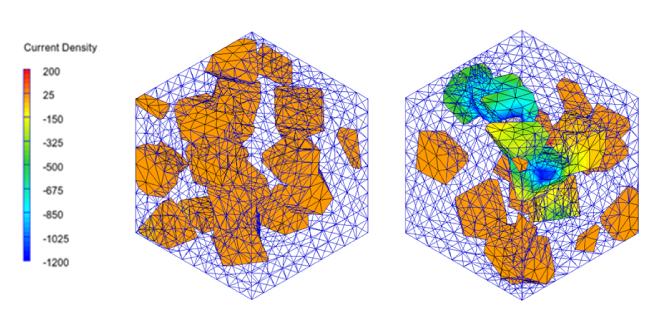 Figure 1. Effects on current distribution and electrical conduction with and without percolation using Digimat
- Link to case study
- Thermal analysis which considers the dispersibility of graphene sheets
2. Ion conduction (diffusion of nanoscale ions) in lithium-ion batteries
In ion conduction, electrical conductivity is determined through analysis of ion diffusion phenomena. For lithium ion batteries, the lithium ion diffusion constant D is used as an index for performance evaluation. The diffusion constant determined from the analysis is converted to mobility µ using Einstein's relation (1), and finally electrical conductivity is obtained.

where kB is the Boltzmann factor and T is the temperature.
By performing a molecular dynamics simulation, the mean square distance (MSD) of a given molecule or atom is determined, and the diffusion constant is obtained from its slope. Figure 2 shows the diffusion constant and electrical conductivity versus mole fraction ratio of an electrolyte solution consisting of LiFSA (lithium bis(fluorosulfonyl)imide), a liquid electrolyte, and propylene carbonate (PC) as a solvent. This result shows that the MSD of Li ions tends to decrease with the electrolyte concentration. This is thought to be because as the proportion of electrolyte increases, reaggregation occurs due to positive and negative ions, which no longer contributes to ion conduction. On the other hand, since electrical conductivity is also proportional to the molar concentration of the electrolyte, this analysis resulted in a gradual increase.
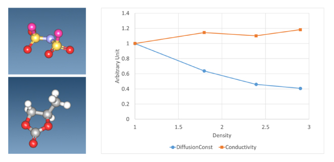 Figure 2. FSA ion (upper left figure) and propylene carbonate (PC) (lower left figure)
Diffusion constant and ionic conductivity of Li ions in LiFSA+PC system for each molar concentration
The ratio of LiFSA and PC is 1:6/1:3/1:2/2:3, and the vertical axis is a dimensionless value normalized to the 1:6 result.
Oxide-based solid electrolytes, along with sulfide-based solid electrolytes, are expected to be used in solid-state batteries, and one candidate is LiZr2(PO4)3 (Figure 3) [3]. As with liquid electrolytes, evaluation of the diffusion constant of Li ions is an indicator for determining ionic conductivity, but unlike liquid electrolytes, which are mainly organic, they are composed of inorganic materials, so it is difficult to analyze using a force field. For this reason, first-principles calculations such as the DFT method are used for analytical evaluation. First-principles calculations are an effective analysis method because once the composition and structure of the object to be analyzed are determined, calculations can proceed without making any assumptions about force fields that include charges (Figure 3). However, the calculation cost is higher than that of classical molecular dynamics calculations, and in particular relaxation calculations for evaluating diffusion constants require analysis on the order of nanoseconds. It is not uncommon for calculations to extend beyond its scale. In recent years, there has been rapid progress in speeding up analysis using machine learning, mainly for inorganic materials, and prediction and evaluation of long-term molecular motion based on machine learning using MD analysis results including first-principles calculations has been rapidly progressing[4].
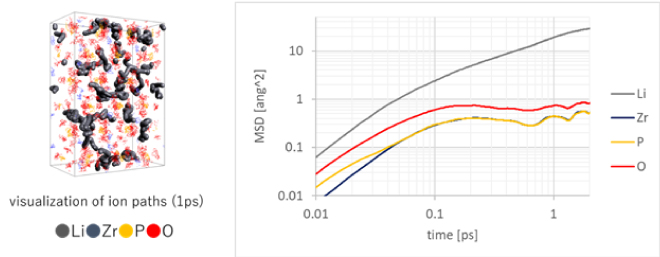 Figure 3. Trajectory of each atom of LiZr2(PO4)3 (thick line is Li ion trajectory) and MSD
(MSD: mean square distance, Li ion mobility evaluation)
3. Hopping conduction (nanoscale/amorphous organic systems)
Hopping conduction is known as an electrical conduction phenomenon in impurities and amorphous materials, and in organic semiconductors such as organic EL, electrons move between molecules (between orbits localized in each molecule) due to hopping conduction (Fig. Four). Although the mobility of hopping conduction is slower than that of band conduction, which will be introduced in the next section, it is thought to be dominant in organic semiconductors [5].
Marcus' theory has long been known as the theory of hopping conduction, and the mobility µ is expressed by the electron transfer speed κ as follows: [6].

Here, t is the transfer integral, λ is the rearrangement energy, ΔG0 is the energy difference between the initial state and the final state, kB is the Boltzmann constant, T is the temperature, and h is the Planck constant. In this regard, the rearrangement energy λ and transfer integral t are calculated using molecular theory [7,8]. As shown in Figure 4 (right) below, λ and ΔG0 are related to the energy curves of the two states before and after electron transfer. Before electron transfer, there are neutral molecules and ionized molecules (E1 in the energy diagram), and after electron transfer, neutral molecules become ionized and molecules in the ionized state become neutral (E2 in the energy diagram). Relocation energy can be calculated from the energy difference between the neutral state and the ionized state. There is a method for calculating the transfer integral based on molecular orbitals [8], and the calculation function is also implemented in ABINIT-MP, which is included with J-OCTA [9]. There is also research in which the mobility calculated in this way was used to calculate the charge movement in a device by dynamic Monte Carlo [10], and it is applied in material development.
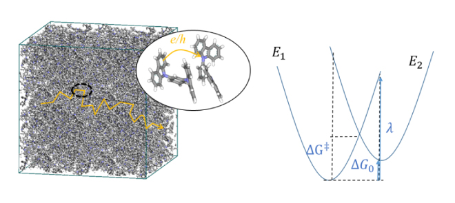 Figure 4. (Left) An image of hopping conduction in organic molecules, (Right) energy curves for the states before (E1) and after (E2) the electron transfer reaction due to hopping.
4. Band conduction (nanoscale/crystal)
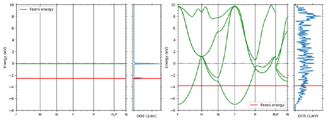
Electrical conduction in inorganic crystals such as metals is called band conduction. Unlike in the previous section, the electrons in these crystals are delocalized and form energy bands that exhibit a wavenumber and energy dispersion relationship that can be considered continuous. There are multiple energy bands for one wave number. The electrical conductivity of a crystal can be confirmed through energy bands. An example is shown in Figure 5. In the metal Cu, the Fermi level intersects with the band curve, and the electrons at the highest level (Fermi level) can be excited to the level immediately above, so it exhibits electrical conductivity. On the other hand, Si, which is an insulator (semiconductor), exists divided into a band completely filled with electrons (valence band) and an empty band above it (conduction band). Due to the existence of this gap, in order for electrons to transition to the conduction band and exhibit conductivity, energy such as heat or light must be applied, or carriers must be introduced through impurities.
The specific expression for the electrical conductivity σ of such materials was given by Drude before the birth of quantum theory. In band conduction, the mobility is

Here, e/m*/τ represent charge, effective mass, and mean free path time, respectively. This formula can also be determined using quantum mechanics, and its validity has been confirmed. From the above equation, the mean free path time τ of electrons is important in determining the electrical conductivity σ, but τ is mainly due to elastic scattering of electrons due to geometrical shapes such as crystal defects and boundaries, and inelasticity due to atomic vibrations. Determined by scattering. Also, the effective mass m* is different from the vacuum electron mass, and is a value that reflects the atomic structure of the crystal. In band theory, it is determined from the curvature of the energy band.
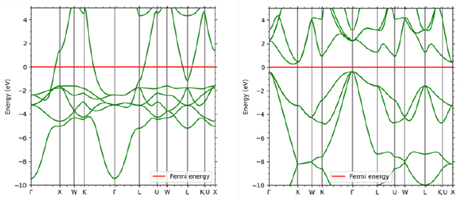 Figure 5. Comparison of band diagrams of Cu (left) and Si (right)

![Figure 7. Analysis example of I-V characteristics of devices that detect various gases (Reference [11])](./img/007/ao007-13.jpg)
![Figure 8. An example of a DNA sequencer analysis model using the NEGF method (Reference [12])Nucleic acid bases used in analysis (a) and placement in nanopores (b to g)](./img/007/ao007-14.jpg)