- Full Atomistic MD
- Optical / Electrical / Magnetic
- Materials Science
[Analysis Example] Dielectric relaxation of polymers
Dielectric relaxation of polymers are calculated using MD.
Objectives and methods
Dielectric relaxation is a means of obtaining information about molecular dynamics from the electrical response of materials. In recent years, the performance of insulating materials used in communication devices has required low dielectric loss, and controlling the dielectric properties of polymers is an important issue.
In this case study, we present an example of dielectric relaxation analysis using autocorrelation function from MD calculation of cis-polybutadiene. An example of analysis with a small molecule system can be found here (case1, case2).
A 25mer polymer model was used, and L-OPLS was specified as the force field. In order to equilibrate the system, NPT calculation was first performed at 500 K. The temperature was decreased at a rate of 10K/1ns, and then NVT calculations were performed at each temperature. The calculations were performed using Gromacs. The autocorrelation function \(\Phi\) of the dipole moment M was calculated from the results, and the relaxation time\(\tau\) was calculated by fitting \(\Phi\) data using the Kohlrausch-Williams-Watts (KWW) equation[1] . Using the parameters obtained from the fitting, we calculated the frequency response by FFT.
\[\Phi(t) = \frac{\langle M(t)M(0) \rangle}{ \langle M(0)M(0) \rangle }\]
\[\Phi_{KWW}(t) = \Phi_{0}exp(-(t/\tau)^\beta)\]
Fig. 1 shows the autocorrelation function \(\Phi\) calculated at each temperature. The fitting of the KWW equation to each data is shown by the black dashed line. In Fig. 2, the relaxation time\(\tau\) obtained by the fitting is plotted against the reciprocal of the temperature, and the values from Ref. [1] are also shown for comparison. Fig. 3 shows the frequency spectrum obtained by the Fourier transform of \(\Phi\)KWW.
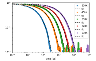 Fig.1: autocorrelation function Φ and fitting result using KWW equation for each temperature.
![Fig.2: The relaxation time tau [ps] obtained from the fitting plotted against 1/T [K-1]](./img/caseA50_img02.jpg) Fig.2: The relaxation time tau [ps] obtained from the fitting plotted against 1/T [K-1]
Fig.2: The relaxation time tau [ps] obtained from the fitting plotted against 1/T [K-1]
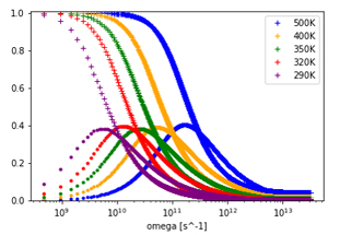 Fig.3: The real and the imaginary part of dielectric relaxation response.